Over the last few months, the Spikefinder challenge has provided a playing ground for colleagues to offer ideas about how to estimate the spiking of individual neurons based on the measured activity of fluorescent calcium indicators.
The challenge was for people to come up with strategies that beat the performance of state-of-the-art algorithms, STM & oopsi. A good number of algorithms were able to achieve this in short time, including one I submitted, termed Vanilla.
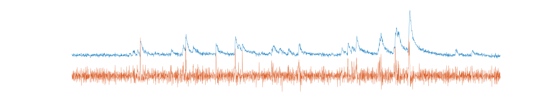
The best performing algorithms seem to have relied on modern machine learning methods. Vanilla is nothing more than a linear filter followed by a static-nonlinearity 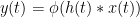
The filter 

The even filter is a Gaussian, 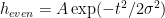


The output nonlinearity is a rectifier to a power, 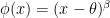

The model has only 4 parameters, 


The model is fit by finding the optimal values of 
The only pre-processing done was a z-scoring of the raw signals. In one dataset (dataset #5, GCaMP6s in V1), we allowed for an extra-delay parameter between the signal and the prediction.
I was surprised this entry did relatively well, as the algorithm it is basically a version of STM. I think the particular shape of the output nonlinearity (rectifier+power vs exponential), the constrain imposed on the shape of the filters, and the resulting small number of parameters, paid a role in Vanilla doing better overall.
The top algorithms reached an absolute performance of about 0.47 and it seems unlikely this performance can be improved by a lot. This seems to highlight the limitations of the current families of calcium indicators in yielding precise spiking information — so there is plenty of opportunity to improve them.
It is interesting that despite its simplicity, the relative performance of Vanilla, with a correlation coefficient of 0.428 was not dramatically inferior to that of the top performing, deep network models, with all its bells and whistles, which landed at 0.464. So, one must pay due respects to deep networks, but I was honestly expecting Vanilla to be completely blown out of the water in terms of performance, and I don’t think it was.
Finally, Vanilla is a non-casual algorithm, as both past and future samples are used to predict the response at time

I’m not convinced that .46 is a true upper bound for the performance. If you look at the deep nets they all overfit substantially. Depending on how correlated the predictions are you could get a better prediction by averaging the predictions from several models (a la bagging), which would get you closer to the true upper bound.
Another point is that the largest improvements were made on datasets which weren’t included in the test set. Look at the scores on dataset 7! It’s the only GCamp6f dataset, and it went from a .55 average between OOPSI and STM to a .8 for most of the deep nets. That’s a pretty large difference – overfitting will eat up a lot of the difference but not all.
There’s no reason you couldn’t train a deep net or the vanilla model in a causal fashion (or causal + buffer) on this problem – I’d be curious to see how much variance you could account for depending on the buffer size.
Point taken — some datasets show large improvements. What I meant is that average performance appeared to asymptote at 0.46 or so for the best performing algorithms. Do you think that could be improved by a lot? Say to 0.55?
There’s no reason you couldn’t train a deep net or the vanilla model in a causal fashion (or causal + buffer) on this problem – I’d be curious to see how much variance you could account for depending on the buffer size.
Yes, that’s exactly what I meant. I’d be an interesting exercise to do.
I think you could raise it to to .5, maybe .55.
The bottleneck is not the amount of data per cell, it’s the number of cells. If you’re building an adaptive algorithm you’re basing it on 173 data points, which is challenging to say the least. I’ve been thinking of ways to augment the data in smart ways to simulate having more data. What if you created virtual cells by adding a random delay to the traces, adding correlated additive + multiplicative, processing with low-pass /high-pass filters, taking mixtures of traces?
Are you writing an xcorr post describing Purgatorio?
I’m writing it up in LaTeX right now for the paper, I might post an HTML version on xcorr.
Hi! I was curious, so I used a random convolutional network and shifted the window that is used for spike predictions by varying delays and measured the performance: http://imgur.com/a/6SHDP (only based on training dataset #1, and not a lot of training, since this is running on a CPU 😉 ). The datapoint with the circle was the setting I had used for the submission. A buffer of 0 (100% causal – right-most data point) seems to be pretty bad, but this may vary between datasets.
Interesting…
Looks promising. A buffer of 10 (second to rightmost) would probably be acceptable, depending on the application. I suspect the results will be a lot better for GCaMP6f than OGB. Try dataset 7.
Same for dataset #7: http://imgur.com/a/eEmWZ
I’m surprised that it seems to be better to let the window rather cover the past than the future, although calcium can only be influenced in the future of the spike. Maybe this should be studied systematically…
Do you have a histogram of beta values? Purgatorio uses beta = 1 and I’m trying to check whether this is reasonable.
There is one beta per dataset, so I have 10 values to share with you… Will send shortly.
Beta values in order of dataset:
1.2193
0.8263
0.7050
2.8254
0.8157
0.4450
0.2967
0.3143
0.8159
1.0324