In addition to tracking the movement of the ball one may want to track eye position along with pupil size. Once again, we use a Dalsa Genie GigE camera to image the eye. Conveniently, it turns out that if you are imaging near 920 nm, there is sufficient light that makes its way through the brain and out of the pupil. Thus, the pupil is clearly visible during imaging and there is no need for additional illumination. The short video below shows one such example of images collected during imaging in primary visual cortex.
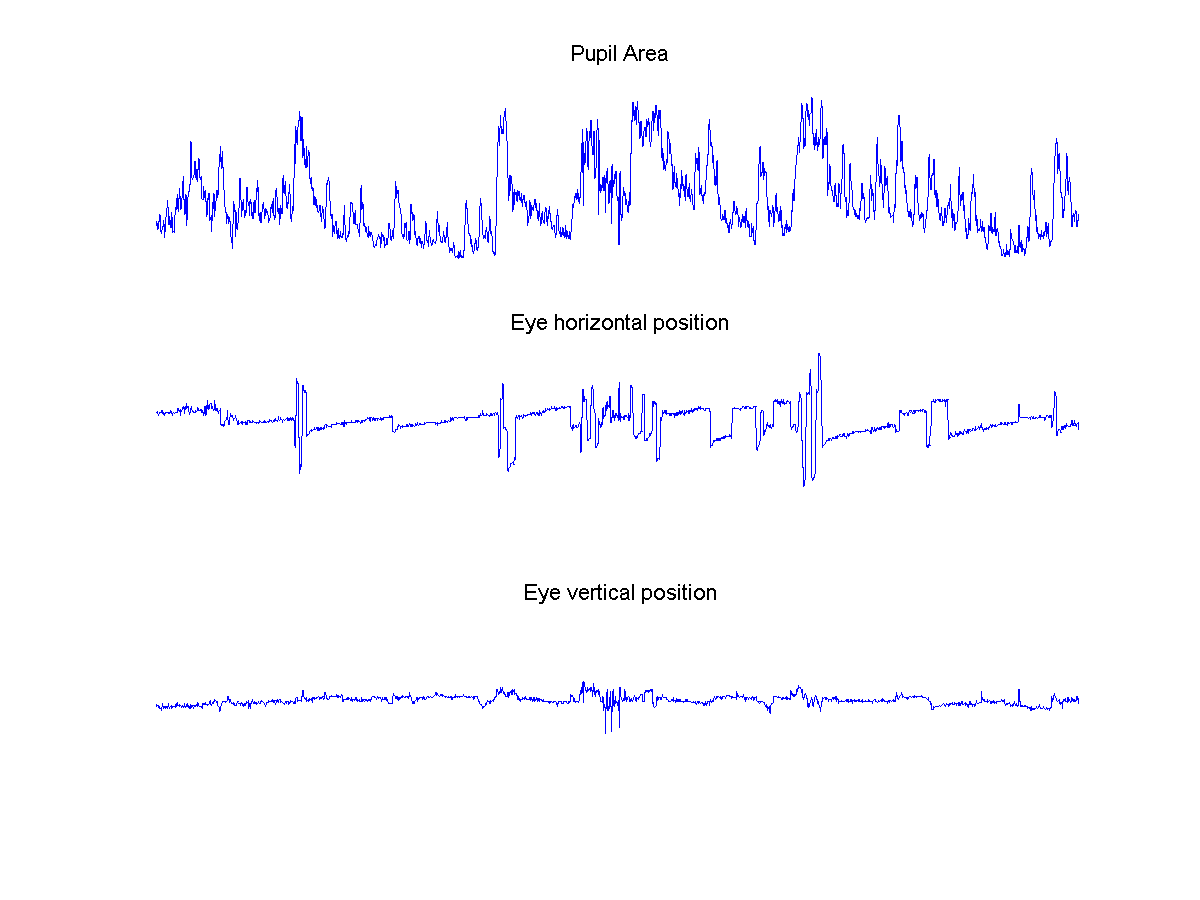
Detecting the center and radius of the pupil is not a difficult task from these data. The biggest obstacles are posed by the occasional movement of the whiskers in front of the eye, blinks and periods of grooming when the eyes are closed and/or occluded. Sample traces of pupil area and eye position obtained are shown below (representing 7 min of data). The parameters are estimated by a straightforward use of Matlab’s imfindcircles function.
As done for the ball tracking, frame acquisition is also triggered by hardware using the Scanbox’s camera synchronization signals. Thus, in our system, the measurements of ball movement, (x,y) eye position, and pupil size, are all synchronized to the frames of the microscope.
The code is based on Matlab’s imfindcircles():
function eye = sbxeyemotion(fn,varargin)</p>
   load(fn,'-mat'); % should be a '*_eye.mat' file

   if(length(varargin)>0)
      rad_range = varargin{1};
   else
      rad_range = [12 32]; % range of radii to search for
   end

   data = squeeze(data); % the raw images...
   xc = size(data,2)/2; % image center
   yc = size(data,1)/2;

   warning off;

   for(n=1:size(data,3))
      [center,radii,metric] = imfindcircles(squeeze(data(yc-W:yc+W,xc-W:xc+W,n)),rad_range,'Sensitivity',1);
      if(isempty(center))
         eye(n).Centroid = [NaN NaN]; % could not find anything...
         eye(n).Area = NaN;
      else
         [~,idx] = max(metric); % pick the circle with best score
         eye(n).Centroid = center(idx,:);
         eye(n).Area = 4*pi*radii(idx)^2;
      end
   end

   save(fn,'eye','-append'); % append the motion estimate data...
