Scanbox includes some basic processing functions that you can use to (a) align the images to compensate for (x,y) movement, (b) segment cells, (c) extract the signals corresponding to the segmented cells from the image sequences.
Motion compensation (sbxalignx & sbxaligndir)
The first step that is sometimes required is to compensate for motion in the (x,y) plane. The basic algorithm we employ was described here. The basic function used to align the images is called sbxalignx().
function [m,T] = sbxalignx(fname,idx)

% Aligns images in fname for all indices in idx
%
% m - mean image after the alignment
% T - optimal translation for each frame
This function takes the name of an image sequence (*.sbx files) and a set of indices (usually from 0 to N-1 where N is the total number of frames in the sequence) and returns an optimal translation for each frame (T) and the mean image of the stack after the alignment (m).
Typically one starts by aligning all experiments, so there is a simple function that will align all the images within a directory called sbxaligndir(). All you have to do is change the working directory in matlab to the one containing the data and simply call sbxaligndir without any arguments. The results are saved in *.align files with the same root name as the original.
Here is what it does:
function sbxaligndir

% Align all *.sbx files in a directory

d = dir('*.sbx');
for(i=1:length(d))
 try
    fn = strtok(d(i).name,'.');
    if(exist([fn '.align'])==0)
       sbxread(fn,1,1);  % read one frame to read the header of the image sequence
       global info;      % this struct contains the information about the structure of the image
       [m,T] = sbxalignx(fn,0:info.max_idx-1); % align the file
       save([fn '.align'],'m','T');            % save the result
       sprintf('Done %s: Aligned %d images in %d min',fn,info.max_idx,round(toc/60))
     else
       sprintf('File %s is already aligned',fn)
     end
 catch
     sprintf('Could not align %s',fn)
 end
end
If you open an *.align file you can check the average, aligned image and the optimal translation for each frame.
>> load -mat fc1_000_001.align
>> figure, imagesc(m),truesize,colormap gray, axis off
>> figure, plot(T)
Once images are aligned
Segmentation (sbxsegmentpoly)
Once the images are aligned one possible way to proceed is to segment the individual cells. There are various semi-automatic ways of doing this published in the literature and we are exploring them. At the moment we are simply manually segmenting the cells using a GUI-based tool that you can call by typing sbxsegmentpoly in the Matlab window.
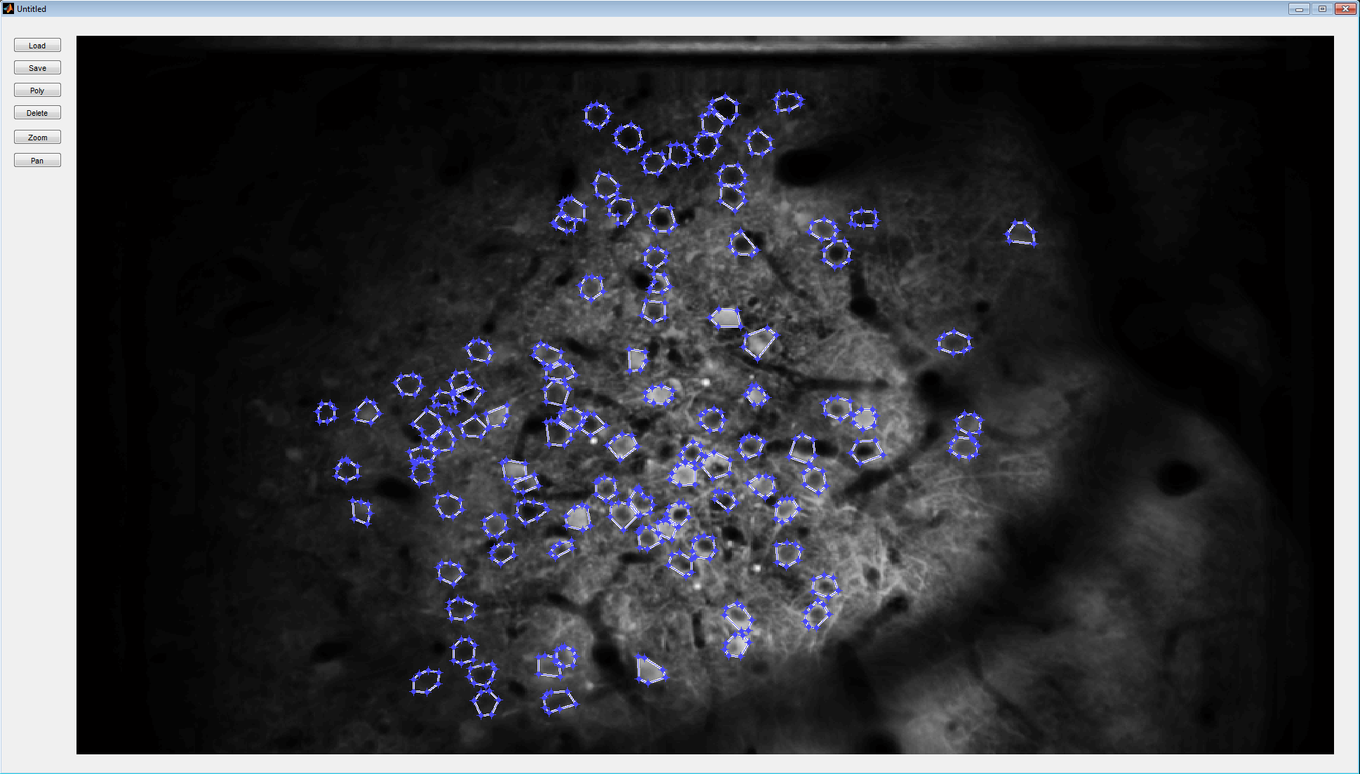
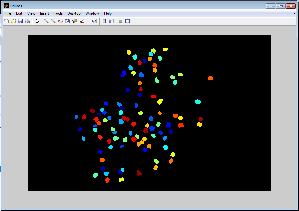
The tool allows you to select arbitrary polygonal regions on the screen that define the cells. Begin by loading an *.align file for an experiment that you have already aligned. You can navigate around the image using the zoom and pan buttons on the top left. When ready to segment a cell hit the button that says “poly”. This will change the cursor on the screen and allow you to click a number of vertices for your polygon. After you trace the boundary of the cell you can close the polygon by double clicking the last vertex. You need to hit “poly” again to segment the next cell… and so on. You can hit “Save” any time during the process to save the areas you have already segmented. If you open an *.align file for which a segmentation was in progress the program will load all the work you have already done. At the end of this manual segmentation process the program generates a corresponding *.segment file that contains the segmentation data. You can visualize the resulting segmentation as follows”
>> load -mat ge7_000_000.segment
>> imshow(label2rgb(mask,'jet','k','shuffle'))
Signal extraction (sbxpullsignals)
Now we are ready to extract the signals for each of the segmented cells from the image sequence. The function sbxpullsignals reads the images, corrects for motion, and extract the mean signal within each of the segmented areas. The result is a matrix with each row corresponding to each of the frames of the sequence and each columns corresponding to each of the cells. This matrix is written into a corresponding *.signals file (the variable is named “sig”) and also returned as the output of the function. Cell #1 (the first column) corresponds to the segmented cell for which mask=1 and so on. So, to plot the activity of cell #10 we simply do:
>> sig = sbxpullsignals('ge7_000_000');  %% this can take time...
>> plot(sig(:,10)), axis off

and zooming in into a segment of the trace:

Now that you have your signals you are ready to start the specific analyses of your experiment.
We will continue to update the tools of this processing pipeline… So stay tuned.
Live long and do good science!
