Patterned photo-stimulation for optogenetics

Scanbox allows patterned photostimulation using a dual galvo pathway.  After installation of the module he first step is to calibrate the system as follows:

1. During installation of the galvo-galvo stimulation module, we will determine the ETL setting required to bring into alignment the 2p imaging plane and the focal plane of stimulation.  This is done by using the port camera to image the scanning area and the stimulation spot simultaneously.  The ETL should be set at this value from this point on.

   

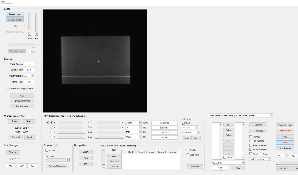
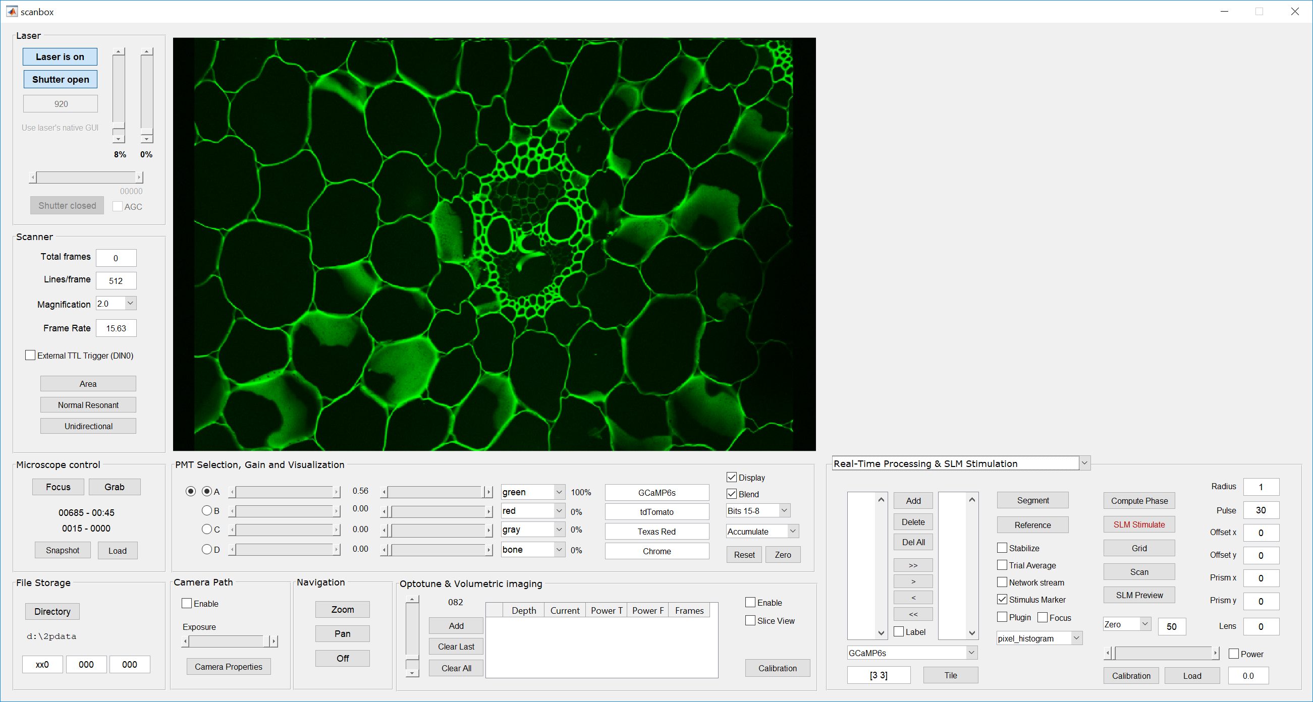
2. We then image a slide that has some fine 2D features, such as a corn stem slide.  Make sure to image at the magnification you want to calibrate.  Calibration has to be performed independently for each magnification.  Use the “accumulate” feature in Scanbox to obtain a nice, average image. Here is an example:

   

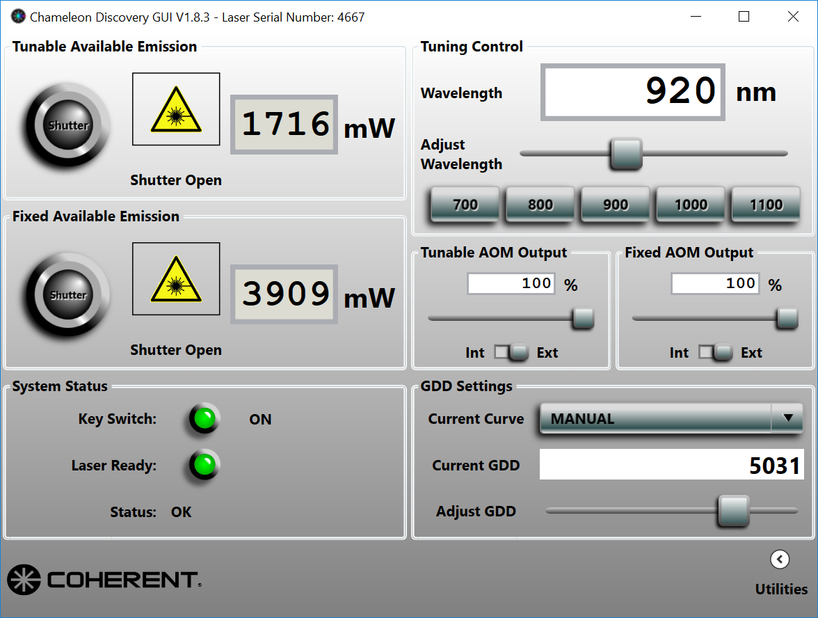
3. Make sure the laser has both shutters open, that the AOM output is set to external and power at 100%.  This allows Scanbox control of the AOM by means of external signals. The panel in the Discovery GUI will should look like this:

   

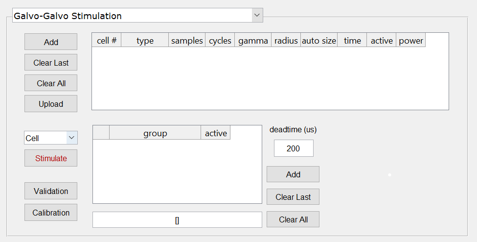
4. In Scanbox, switch to the Galvo-galvo panel and you will see a “Calibration” button on the bottom left corner.  Press the button and the calibration process will start.

   

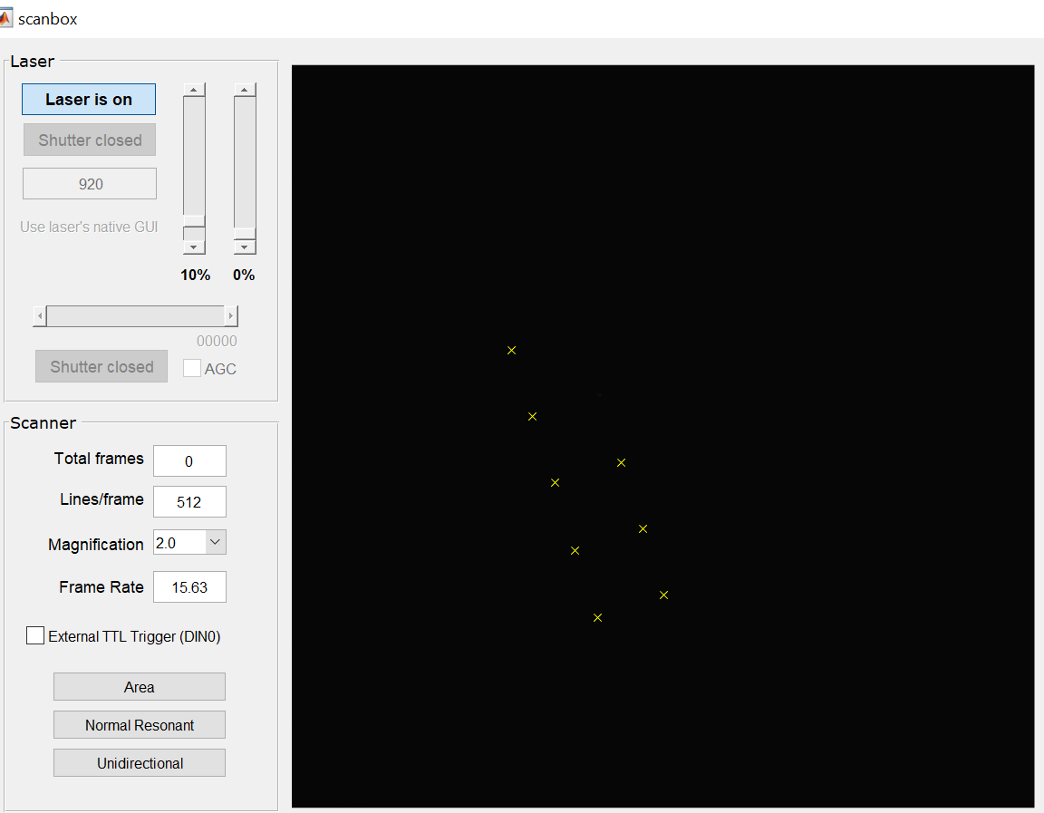
5. The system will move the camera mirror in place and take a camera view of the sample. It will then proceed to display a spot at several grid locations.  As these spots are detected, a ‘x’ mark will be left behind. The figure below shows one snapshot while the system was collecting data on a 5×5 grid.

   

6. When Scanbox finishes collecting these data it will present you with two images in Matlab’s control point selection tool.  This allows you to select matching features in the two images.  The image on the left is the image of the sample via the port camera (which, at the moment, it must be a PCO camera).  The image on the right displays the two-photon image acquired in step #1.  You can proceed by selecting matching points on both images.  We typically collect ~20-25 points distributed cross the field of view. Here is an example at the end of this process:

   
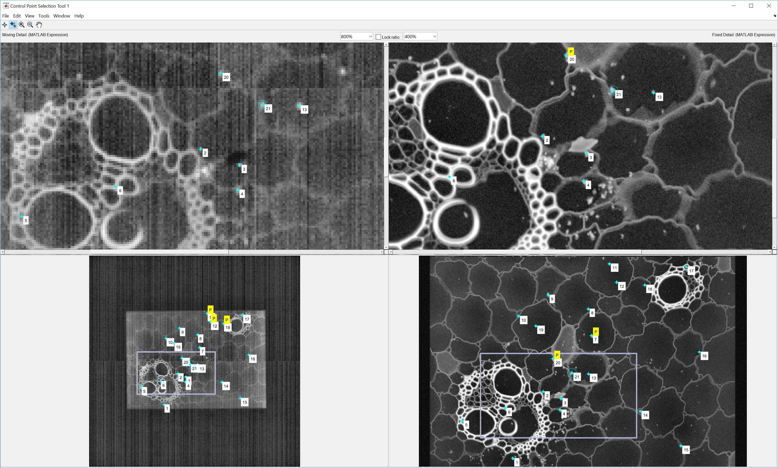
   You can use the selection tool prediction features to check you have sufficient points to allow a good match between the two images.  Once the prediction feature is turned on, selecting a feature on one image will automatically display the predicted match on the second one.   Once satisfied with the selected points, do File->Close in the Control Point Selection GUI.  Scanbox will now ask you to save the calibration in a file.  Provide a name and save it.

The above process is all that is needed to calibrate the system.  To check everything is working as intended place a green slide under the objective and focus about 150 um below the surface we can now proceed to do a validation by making small holes in the slide as follows:

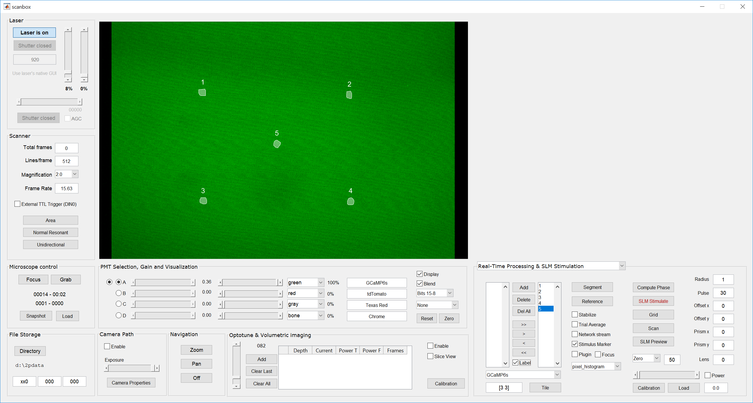
1. Define a small number of ROIs in Scanbox (around 5-10).  You do this in the “Real-Time Processing” panel.  Click the “Label” checkbox to display their numbers as well.
   
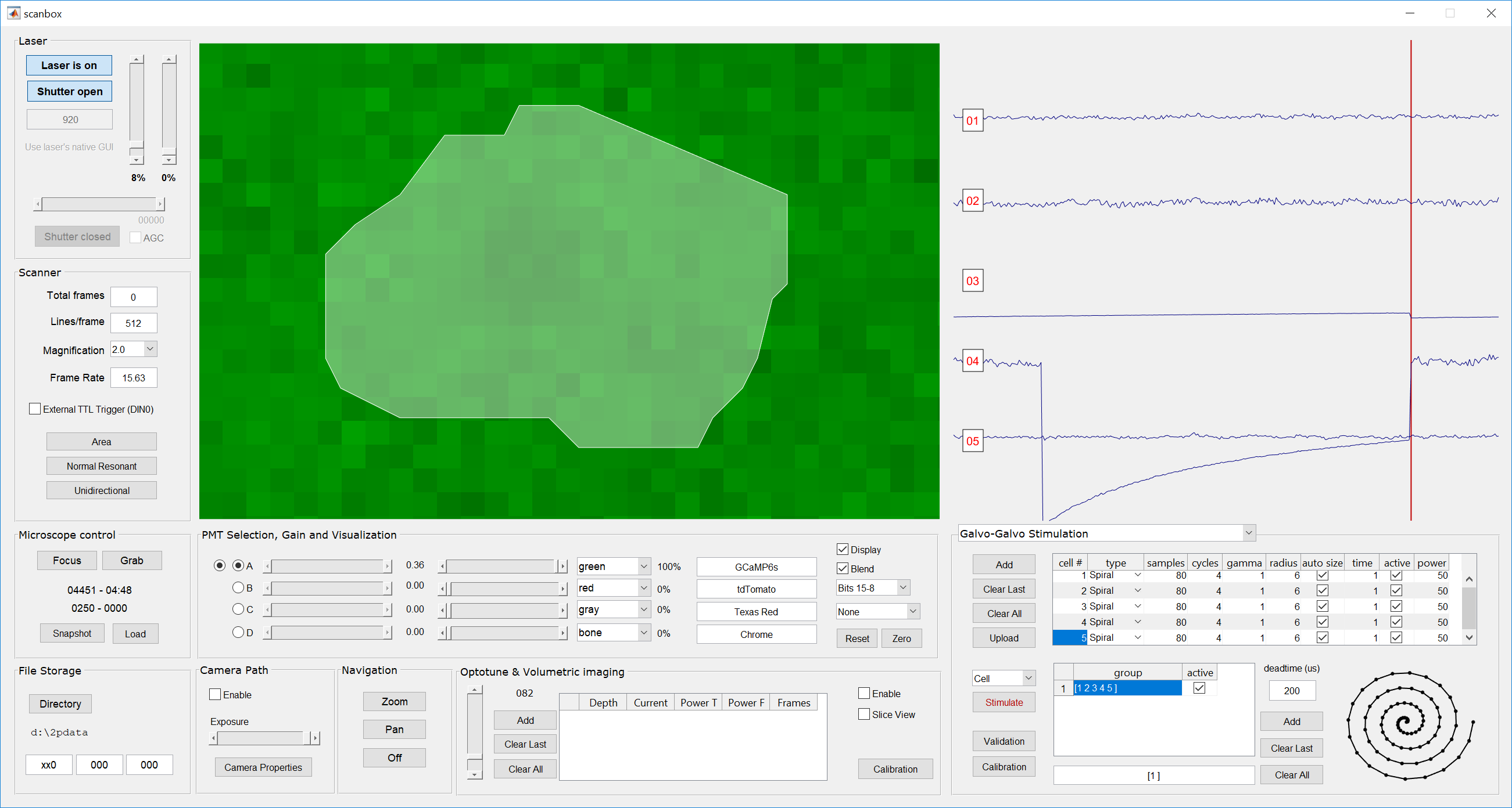
2. Switch to the Galvo-galvo stimulation panel and add the same number of cells as defined in step #1 using the “Add” button on the top left.  You will see a spreadsheet-like table being populated with the cell numbers and stimulation parameters for each.  Leave everything with their default values.

   

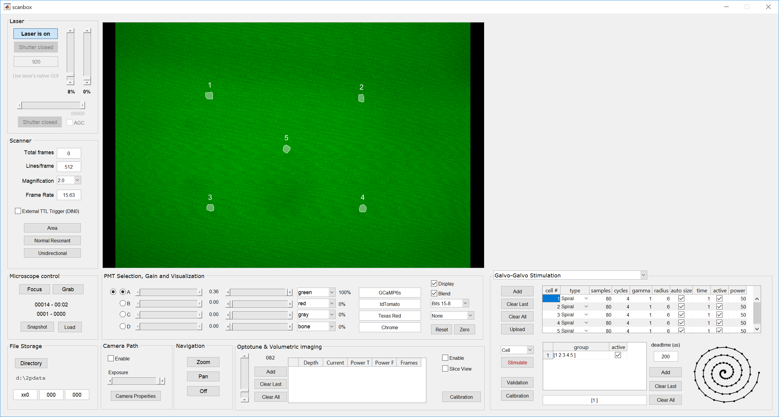
3. Once a few cells are defined we can now define groups of neurons.  Click the “Add” button on the group definition section, which is to the right of the group spreadsheet.  You will see a group defined as [1 2 3 4 5] and, at the bottom, a field defined [1].  This field is called the Protocol field.  Click on the “Upload” button to send all the stimulation parameters to the box.Note that a group is a sequence of cells, while a protocol is a sequence of groups.  Scanbox allows you to stimulate cells, groups or protocols.  A pull down menu above the “Stimulate” button allows you to select which type you want.  You select a cell or a group by clicking on the desired row.  For example, the picture above shows cell #1 selected and “Cell” stimulation is shown in the pull-down menu.  If we click “Stimulate” the system will stimulate cell #1 with the parameters defined.
4. Start scanning and use and stimulate each of the ROIs.  After ~5 stimulation pulses you may see a faint black dot near the ROI you selected.  As soon as the spot is barely visible stop and move to the next location.  When you have made holes in all your ROIs you can stop scanning and use the “Zoom” and “Pan” buttons in the navigation panel to take a close look to assess if the center of the ROI aligns with the stimulation bubbles.  Here is an example showing good alignment.

   
   If your micro-bubbles align well with the center of the ROIs you are now ready to go!  If there is a systematic shift in the alignment you can use the ggs_x_bias and ggs_y_bias configuration variables to correct them.

Pattern definition

In principle, each cell can be stimulated with a different pattern.  A pattern consists of a sequence of (x,y) locations.  These points are stimulated in sequence at a rate of 80kHz.  That means that a pattern with 80 points will be shown in 1 ms.  This rate is fixed and not under user control.  Thus, if you want shorter or longer stimulation periods you need to change the number of points in the pattern. Patterns type can be selected with a pull-down menu.  At the moment there are only two types, spiral and Thomson.

A spiral pattern is shown below.  the user can change the number of samples, the total number of cycles around the circle with those points and a gamma parameter that controls how much the points are concentrated near the boundary.  The radius of the pattern is defined in pixels and can be automatically detected whether cells are defined using the on-line cell selection tool or defined manually.  As the parameters are modified, the new pattern is displayed graphically within the panel on the bottom right to provide visual feedback.

Cells can also be active or not.  So, after defining cells, groups and protocols, if one wants just to drop a cell all you have to do is deselect the “active” checkbox.  That will remove the cell from groups and protocols.  Similarly, a group can be made active or not buy clicking its “active” checkbox.

A Thompson pattern is computed by simulating the placement of random dots within the unit circle and letting them repel each other as if they were charged particles.  The points evolve to minimize the potential.  The gamma variable again determines how concentrated the points will be near the boundary.  Points in the Thompson pattern are presented in a random sequence during stimulation.

Here is an example of such a pattern for gamma=1.  Thompson patterns are computed in real time and the points appear red during the calculation.  Please wait until convergence, when the points turn black, to add your next pattern or changing the parameters.

The deadtime field allows selection of a deadtime between patterns.  Note that the stimulation of cells, groups and protocols are synchronized to the beginning of the 2p frame scan.  If a stimulation command arrives in the middle of a frame, Scanbox will wait until the beginning of the next frame to trigger the stimulation.

Shortest scan path

Once a group is defined its members will be stimulated in order by default.  Alternatively, one can select a group and click the “Shortest Path” button to have the members re-ordered to produce the shortest scan path for stimulation.  The shortest path will be displayed on the screen.

Configuration variables

The main configuration variables you may want to change are ggsscal, which determines the calibration file loaded when Scanbox starts up; ggs_nx and ggs_ny, which determine the number of points in the calibration grid; ggs_x_bias and ggs_y_bias are in pixels and used to compensate for any systematic shifts observed in the validation step.

sbconfig.ggs = true; % gg stim option

sbconfig.ggscal = 'ggx2.mat'; % default ggcal calibration file

sbconfig.ggs_width = 8; % in volts!
sbconfig.ggs_height = 8;

sbconfig.ggs_nx = 5; % # of points in calibration grid in x and y - must be odd!
sbconfig.ggs_ny = 5;

sbconfig.ggs_power = 0.07; % power as a fraction of max laser power

sbconfig.ggs_xval = 796/4 * [1 2 3]; % validation points
sbconfig.ggs_yval = 512/4 * [1 2 3];
sbconfig.ggs_val_power = .8; % validation power (for holes!)
sbconfig.ggs_val_delay = .02; % validation power (for holes!)
sbconfig.ggs_val_trials = 1;

sbconfig.ggs_x_bias = -6; % calibration bias in pixels
sbconfig.ggs_y_bias = 0;

Network commands

Network commands allow the selection of stimulation type (cell, group or protocol) and remote stimulation.

To remotely change stimulus type use “gm <type> <index>” to select a stimulus type and index. The stimulus type is 1 (cell), 2 (group) or 3 (protocol). For the first two cases an index is needed which points to an entry in the corresponding table. For cell selection, the index will select on of the cells in the pattern definition table. For group selection, the index will select one of the groups of in the group definition table. The stimulation type pull-down menu will reflect the selected mode and the first cell of the table selection will be highlighted.

To remotely trigger the selected stimulus you can simply send a “gs” command. This is equivalent to hitting the “Stimulate” button in the galvo-galvo stimulation panel.

To remotely enable/disable the hardware trigger (see next section) use “gt <val>” You can disable the trigger with a value of 0 and enable with 1.

External trigger

Once cells, groups and protocols have been defined and a mode selected , one can externally trigger the stimulation with the rising edge of a TTL signal input to PSoC 2, DIN_1. This can be enabled manually through the checkbox in the panel or remotely (see previous section). If you want this TTL signal time-stamped you will need to route it also to one of the TTL EVENTS inputs on PSoC 1.

Automatic PMT gating

A PMT gate signal is generated automatically by Scanbox during stimulation, so there is no need for any additional, external logic.